Background Reading: How do we analyze spatial dispersion?
In Figure 8.4 the three dispersion patterns are readily distinguished. However, in practice, categorizing the dispersion pattern is not always so easy, because the three patterns grade into one another. Thus it is important to be able to quantitatively assign a dispersion pattern to a population.
One important method for answering this question is based on the statistical distribution pattern known as the Poisson distribution. The Poisson distribution is a random pattern that applies to relatively rare events. We compare the actual pattern of distribution to this theoretical random dispersion. If they match, the dispersion pattern is random. If not, the dispersion pattern is either clumped or regular.
To use this method, a grid is laid over the dispersion pattern of the population such that the mean number of individuals in each grid square is small. In Figure 8.6 the grid results in a mean of 0.51 individuals per square. As you see in the figure, some have 0 individuals, some have 1, some have 2, and so on. We calculate the expected number of grid squares with certain numbers of individuals under the Poisson (random) distribution.
The expected proportion of squares with x individuals is calculated with the formula
where is the number of occurrences, is the mean number of occurrences per grid square, and is the base of the natural logarithms. The value is known as “ factorial.” This means that we multiply the value times the values , , , and so on, until the remaining term is 1. For example, . The expected number of squares with individuals is then calculated by multiplying the expected proportion of squares by the total number of squares.
For example, the expected proportion of squares with 2 individuals is
We can now calculate the expected number of squares containing 2 individuals by multiplying the expected proportion by the total number of squares, in this example 100:
Thus we expect 7.8 squares to contain 2 individuals if the dispersion is random. We do similar calculations for each expected number up to the maximum number observed. As discussed in the text we can use the chi square statistical test to determine if the observed values differ significantly from the expected values.
There is another important way we can evaluate the Poisson analysis. One important characteristic of a Poisson distribution is that the mean number of events (in this case individuals per grid square) equals the variance in the number of events. Thus, if the dispersion is random, the mean/variance ratio should be 1.0. However, if the distribution is clumped, the grid squares differ markedly in the number of individuals they contain—some have none whereas others have many. In other words, the variance in the number per square is high. In this case the mean/variance ratio is small, less than 1.0. This contrasts with the situation in the regular dispersion pattern, in which each square holds about the same number of individuals. In this case the variation is small and the mean/variance ratio is greater than 1.
For additional background information, please see Section 8.2 in Chapter 8, "How Do We Measure the Spatial Distribution of Individuals in a Population?"
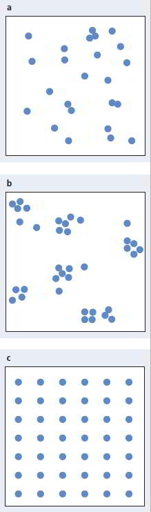
Figure 8.4 Dispersion patterns. There are three possible dispersion patterns: (a) random, (b) clumped, and (c) regular.