Background reading part 1: How Do Birth and Death Rates Determine the Growth Rate of a Population?
The birth and death rates are the two key internal factors in the dynamics of a population. The age-specific changes in these factors are found in life table data (see the Living Graph exercise on Survivorship Curves). When dispersing individuals occupy a new and suitable habitat, the population grows exponentially. A small population in exponential growth initially increases slowly, but over time the rate of growth increases (see Figure 8.16). Of course, the population cannot grow indefinitely; a number of factors eventually reduce the growth rate. If we are to understand the dynamics of populations the limits to growth, it is important that we analyze the mathematics of population growth.
We mathematically characterize exponential growth in two ways depending on the reproductive pattern of the species. Consider a population of annual plants that doubles each year. The population in the next year, time , is calculated from the population at time as follows:
The variable is the multiplicative growth rate, the factor by which the population increases in each time period. For this population, . We calculate the population at any time from and the starting population, :
Recall that we can also use the net reproductive rate, , the expected number of offspring a female produces in her lifetime, in a similar way:
The situation is more complex for species with overlapping generations. In any reproductive season, some of the individuals reproducing will be young individuals reproducing for the first time. Others will be older individuals who have reproduced in previous seasons and survived to the current one. To model this kind of growth we begin with the equation
The change in the population, , is calculated
If , we can calculate by subtracting from both sides of the equation,
Then
Notice that if the value of D exceeds the value of B, the change in the population (ΔN) is negative. Moreover, the values of B and D change with the population size. To account for this we use per capita measures of birth and death (b) and (d). This changes the equation to
And the change in the population becomes
In order to express growth as an instantaneous change, we use the differential equation
And we replace with a new variable, , the instantaneous growth rate (also known as the intrinsic rate of increase):
Now we can derive a general equation for population growth:
where e is the base of the natural logarithms. Note that when , the equation becomes . In this case we can rewrite this equation using :
For additional background information, please see Section 8.3 of Chapter 8, How doe Populations with Discrete Generations Grow? and How Do Populations with Overlapping Generations Grow?
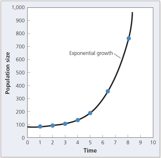
Figure 8.16 Exponential growth. When a population is introduced into new, suitable habitat, it often grows exponentially.