Background reading: How do stochastic events affect allele frequencies?

If, for example, we expect homozygous dominants to occur with the frequency $p^{2}$ , it is entirely possible that the actual frequency will be lower or higher than this value simply by chance. The phenomenon is more pronounced in small populations. Consider the analogy of flipping a coin. We expect 50 percent heads and 50 percent tails. But if you flip a coin only four times, it's entirely possible to get three heads and a tail or even four heads and no tails just by chance. It is far less likely to obtain all heads if you flip the coin 100 times. A number of factors contribute to chance deviation from expectations. However, all are the result of some factor that causes the population to depart from purely random mating in which the laws of probability play out as expected. We define the effective population size ( $N_{e}$ ) as the subset of the total population that mates randomly. Any characteristic of the population that reduces random mating reduces the effective population size. As $N_{e}$ becomes smaller than the actual population size, drift becomes more pronounced. For example, if the sex ratio, the proportion of the population that is male and female, is heavily skewed toward one sex, the population will not behave like a large, randomly mating group. Consider a population of 100 individuals. If 90 are female and only 10 are male, those few males must mate with all the females to produce the next generation. In effect the population is not 100 randomly mating individuals; all the offspring are the product of just 10 males, and because of their small numbers, chance events will skew their genetic contribution, leading to shifts in allele frequency.

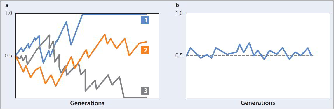
The first graph plots allele frequency from 0 to 1.0, versus generations for three populations. Population 1: Starts at 0.5, has many serrations, then rises and plateaus at 1. Population 2: Starts at 0.5, falls, rises, and ends at 0.7. Population 3: Starts at 0.5, rises, falls, and then plateaus at 0. The second graph plots 0 to 1.0 versus generations. There is a horizontal dotted line at 0.5. The graph is a slightly serrated line that slightly goes up and down the horizontal line.

Figure 2.13 Genetic drift. The effects of genetic drift are more pronounced in small populations (a) than in large populations (b). In (a) each line represents a single, small population. In population 1, drift led to fixation of the allele. Population 3 lost the allele. In population 2, the allele persisted until the end of the experiment.

If we follow a series of populations in which drift occurs over time, some reach a $p$ value of 1.0 whereas others fall to 0 (see Figure 2.13). When $p = 1.0$ the recessive allele has been lost. In this case we say that the dominant allele has become fixed. Similarly, when $p = 0$ the dominant allele has been lost and the recessive has been fixed. Loss and fixation of alleles are the inevitable consequence of genetic drift. Because drift is a random process, it is unpredictable whether any particular allele will be lost or fixed. But given enough time, one or the other will occur (see Figure 2.14).

For additional background information, see Section 2.3 of Chapter 2 in your textbook, How Does Genetic Drift Change Allele Frequencies?

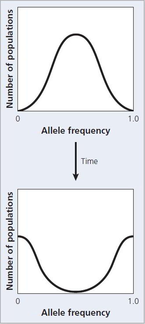
The first graph plots number of populations versus allele frequency from 0 to 1.0. The graph has a normal distribution. After a period of time, the second graph plots number of populations versus allele frequency from 0 to 1.0. The graph is now a U shape.

Figure 2.14 Genetic drift leads inevitably to the loss or fixation of alleles. Over time, a group of populations will shift from a normal distribution of allele frequencies to populations in which the allele has either been fixed or lost.